Hướng dẫn scatter plot multiple variables python - phân tán biểu đồ nhiều biến python

Scatter plot is a graph in which the values of two variables are plotted along two axes. It is a most basic type of plot that helps you visualize the relationship between two variables.

Concept

1. What is a Scatter plot?
2. Basic Scatter plot in python
3. Correlation with Scatter plot
4. Changing the color of groups of points
5. Changing the Color and Marker
6. Scatter plot with Linear fit plot using seaborn
7. Scatter Plot with Histograms using seaborn
8. Bubble plot
9. Exploratory Analysis using mtcars Dataset
   • Multiple line of best fits
   • Adjusting color and style for different categories
   • Text Annotation in Scatter Plot
   • Bubble Plot with categorical variables
   • Categorical Plot

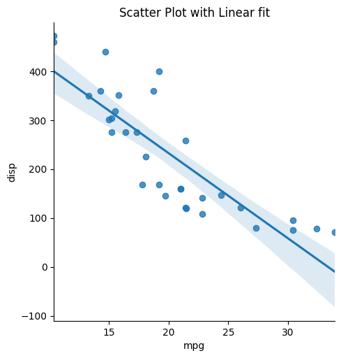
What is a Scatter plot?

Scatter plot is a graph of two sets of data along the two axes. It is used to visualize the relationship between the two variables.

If the value along the Y axis seem to increase as X axis increases(or decreases), it could indicate a positive (or negative) linear relationship. Whereas, if the points are randomly distributed with no obvious pattern, it could possibly indicate a lack of dependent relationship.

In python matplotlib, the scatterplot can be created using the

# Simple Scatterplot
x = range(50)
y = range(50) + np.random.randint(0,30,50)
plt.scatter(x, y)
plt.rcParams.update({'figure.figsize':(10,8), 'figure.dpi':100})
plt.title('Simple Scatter plot')
plt.xlabel('X - value')
plt.ylabel('Y - value')
plt.show()

# Simple Scatterplot with colored points
x = range(50)
y = range(50) + np.random.randint(0,30,50)
plt.rcParams.update({'figure.figsize':(10,8), 'figure.dpi':100})
plt.scatter(x, y, c=y, cmap='Spectral')
plt.colorbar()
plt.title('Simple Scatter plot')
plt.xlabel('X - value')
plt.ylabel('Y - value')
plt.show()

So what is the difference between

# Simple Scatterplot with colored points
x = range(50)
y = range(50) + np.random.randint(0,30,50)
plt.rcParams.update({'figure.figsize':(10,8), 'figure.dpi':100})
plt.scatter(x, y, c=y, cmap='Spectral')
plt.colorbar()
plt.title('Simple Scatter plot')
plt.xlabel('X - value')
plt.ylabel('Y - value')
plt.show()

# Simple Scatterplot with colored points
x = range(50)
y = range(50) + np.random.randint(0,30,50)
plt.rcParams.update({'figure.figsize':(10,8), 'figure.dpi':100})
plt.scatter(x, y, c=y, cmap='Spectral')
plt.colorbar()
plt.title('Simple Scatter plot')
plt.xlabel('X - value')
plt.ylabel('Y - value')
plt.show()

The difference between the two functions is: with

# Simple Scatterplot
x = range(50)
y = range(50) + np.random.randint(0,30,50)
plt.scatter(x, y)
plt.rcParams.update({'figure.figsize':(10,8), 'figure.dpi':100})
plt.title('Simple Scatter plot')
plt.xlabel('X - value')
plt.ylabel('Y - value')
plt.show()

# Simple Scatterplot with colored points
x = range(50)
y = range(50) + np.random.randint(0,30,50)
plt.rcParams.update({'figure.figsize':(10,8), 'figure.dpi':100})
plt.scatter(x, y, c=y, cmap='Spectral')
plt.colorbar()
plt.title('Simple Scatter plot')
plt.xlabel('X - value')
plt.ylabel('Y - value')
plt.show()

That is, in

# Simple Scatterplot with colored points
x = range(50)
y = range(50) + np.random.randint(0,30,50)
plt.rcParams.update({'figure.figsize':(10,8), 'figure.dpi':100})
plt.scatter(x, y, c=y, cmap='Spectral')
plt.colorbar()
plt.title('Simple Scatter plot')
plt.xlabel('X - value')
plt.ylabel('Y - value')
plt.show()

# Simple Scatterplot
x = range(50)
y = range(50) + np.random.randint(0,30,50)
plt.scatter(x, y)
plt.rcParams.update({'figure.figsize':(10,8), 'figure.dpi':100})
plt.title('Simple Scatter plot')
plt.xlabel('X - value')
plt.ylabel('Y - value')
plt.show()

First, I am going to import the libraries I will be using.

import pandas as pd
import numpy as np
import matplotlib.pyplot as plt
%matplotlib inline
plt.rcParams.update({'figure.figsize':(10,8), 'figure.dpi':100})

The

# Simple Scatterplot with colored points
x = range(50)
y = range(50) + np.random.randint(0,30,50)
plt.rcParams.update({'figure.figsize':(10,8), 'figure.dpi':100})
plt.scatter(x, y, c=y, cmap='Spectral')
plt.colorbar()
plt.title('Simple Scatter plot')
plt.xlabel('X - value')
plt.ylabel('Y - value')
plt.show()

Basic Scatter plot in python

First, let’s create artifical data using the

# Simple Scatterplot with colored points
x = range(50)
y = range(50) + np.random.randint(0,30,50)
plt.rcParams.update({'figure.figsize':(10,8), 'figure.dpi':100})
plt.scatter(x, y, c=y, cmap='Spectral')
plt.colorbar()
plt.title('Simple Scatter plot')
plt.xlabel('X - value')
plt.ylabel('Y - value')
plt.show()

You can also specify the lower and upper limit of the random variable you need.

Then use the

# Simple Scatterplot with colored points
x = range(50)
y = range(50) + np.random.randint(0,30,50)
plt.rcParams.update({'figure.figsize':(10,8), 'figure.dpi':100})
plt.scatter(x, y, c=y, cmap='Spectral')
plt.colorbar()
plt.title('Simple Scatter plot')
plt.xlabel('X - value')
plt.ylabel('Y - value')
plt.show()

# Scatterplot of non-random vzriables
x=np.arange(1,10,0.2)
y= np.exp(x)
plt.scatter(x,y)
plt.rcParams.update({'figure.figsize':(10,8), 'figure.dpi':100})
plt.title('Exponential Relation dataset')
plt.show()

# Scatterplot of non-random vzriables
x=np.arange(1,10,0.2)
y= np.exp(x)
plt.scatter(x,y)
plt.rcParams.update({'figure.figsize':(10,8), 'figure.dpi':100})
plt.title('Exponential Relation dataset')
plt.show()

# Scatterplot of non-random vzriables
x=np.arange(1,10,0.2)
y= np.exp(x)
plt.scatter(x,y)
plt.rcParams.update({'figure.figsize':(10,8), 'figure.dpi':100})
plt.title('Exponential Relation dataset')
plt.show()

Get Free Complete Python Course

Facing the same situation like everyone else?

Build your data science career with a globally recognised, industry-approved qualification. Get the mindset, the confidence and the skills that make Data Scientist so valuable.

Get Free Complete Python Course

Build your data science career with a globally recognised, industry-approved qualification. Get the mindset, the confidence and the skills that make Data Scientist so valuable.

# Simple Scatterplot
x = range(50)
y = range(50) + np.random.randint(0,30,50)
plt.scatter(x, y)
plt.rcParams.update({'figure.figsize':(10,8), 'figure.dpi':100})
plt.title('Simple Scatter plot')
plt.xlabel('X - value')
plt.ylabel('Y - value')
plt.show()

You can see that there is a positive linear relation between the points. That is, as X increases, Y increases as well, because the Y is actually just X + random_number.

If you want the color of the points to vary depending on the value of Y (or another variable of same size), specify the color each dot should take using the

# Scatterplot of non-random vzriables
x=np.arange(1,10,0.2)
y= np.exp(x)
plt.scatter(x,y)
plt.rcParams.update({'figure.figsize':(10,8), 'figure.dpi':100})
plt.title('Exponential Relation dataset')
plt.show()

You can also provide different variable of same size as X.

# Simple Scatterplot with colored points
x = range(50)
y = range(50) + np.random.randint(0,30,50)
plt.rcParams.update({'figure.figsize':(10,8), 'figure.dpi':100})
plt.scatter(x, y, c=y, cmap='Spectral')
plt.colorbar()
plt.title('Simple Scatter plot')
plt.xlabel('X - value')
plt.ylabel('Y - value')
plt.show()

Lets create a dataset with exponentially increasing relation and visualize the plot.

# Scatterplot of non-random vzriables
x=np.arange(1,10,0.2)
y= np.exp(x)
plt.scatter(x,y)
plt.rcParams.update({'figure.figsize':(10,8), 'figure.dpi':100})
plt.title('Exponential Relation dataset')
plt.show()

# Scatterplot of non-random vzriables
x=np.arange(1,10,0.2)
y= np.exp(x)
plt.scatter(x,y)
plt.rcParams.update({'figure.figsize':(10,8), 'figure.dpi':100})
plt.title('Exponential Relation dataset')
plt.show()

Now you can see that there is a exponential relation between the x and y axis.

Correlation with Scatter plot

1) If the value of y increases with the value of x, then we can say that the variables have a positive correlation.

2) If the value of y decreases with the value of x, then we can say that the variables have a negative correlation.

3) If the value of y changes randomly independent of x, then it is said to have a zero corelation.

# Scatterplot and Correlations
# Data
x=np.random.randn(100)
y1= x*5 +9 
y2= -5*x
y3=np.random.randn(100)

# Plot
plt.rcParams.update({'figure.figsize':(10,8), 'figure.dpi':100})
plt.scatter(x, y1, label=f'y1 Correlation = {np.round(np.corrcoef(x,y1)[0,1], 2)}')
plt.scatter(x, y2, label=f'y2 Correlation = {np.round(np.corrcoef(x,y2)[0,1], 2)}')
plt.scatter(x, y3, label=f'y3 Correlation = {np.round(np.corrcoef(x,y3)[0,1], 2)}')

# Plot
plt.title('Scatterplot and Correlations')
plt.legend()
plt.show()

In the above graph, you can see that the blue line shows an positive correlation, the orange line shows a negative corealtion and the green dots show no relation with the x values(it changes randomly independently).

Changing the color of groups of points

Use the

# Scatterplot of non-random vzriables
x=np.arange(1,10,0.2)
y= np.exp(x)
plt.scatter(x,y)
plt.rcParams.update({'figure.figsize':(10,8), 'figure.dpi':100})
plt.title('Exponential Relation dataset')
plt.show()

# Scatterplot - Color Change
x = np.random.randn(50)
y1 = np.random.randn(50)
y2= np.random.randn(50)

# Plot
plt.scatter(x,y1,color='blue')
plt.scatter(x,y2,color= 'red')
plt.rcParams.update({'figure.figsize':(10,8), 'figure.dpi':100})

# Decorate
plt.title('Color Change')
plt.xlabel('X - value')
plt.ylabel('Y - value')
plt.show()

Changing the Color and Marker

Use the

# Scatterplot of non-random vzriables
x=np.arange(1,10,0.2)
y= np.exp(x)
plt.scatter(x,y)
plt.rcParams.update({'figure.figsize':(10,8), 'figure.dpi':100})
plt.title('Exponential Relation dataset')
plt.show()

[‘.’,’o’,’v’,’^’,’>’,'&lt;‘,’s’,’p’,’*’,’h’,’H’,’D’,’d’,’1′,”,”] – These are the types of markers that you can use for your plot.<p></p> <pre><code class="lang-python"><span class="hljs-comment"># Scatterplot of different distributions. Color and Shape of Points.</span> x = np.random.randn(<span class="hljs-number">500</span>) y1 = np.random.randn(<span class="hljs-number">500</span>) y2 = np.random.chisquare(<span class="hljs-number">10</span>, <span class="hljs-number">500</span>) y3 = np.random.poisson(<span class="hljs-number">5</span>, <span class="hljs-number">500</span>) # Plot plt.rcParams.update({<span class="hljs-string">'figure.figsize'</span>:(<span class="hljs-number">10</span>,<span class="hljs-number">8</span>), <span class="hljs-string">'figure.dpi'</span>:<span class="hljs-number">100</span>}) plt.scatter(x,y1,color=<span class="hljs-string">'blue'</span>, marker= <span class="hljs-string">'*'</span>, <span class="hljs-keyword">label</span><span class="bash">=<span class="hljs-string">'Standard Normal'</span>) </span>plt.scatter(x,y2,color= <span class="hljs-string">'red'</span>, marker=<span class="hljs-string">'v'</span>, <span class="hljs-keyword">label</span><span class="bash">=<span class="hljs-string">'Chi-Square'</span>) </span>plt.scatter(x,y3,color= <span class="hljs-string">'green'</span>, marker=<span class="hljs-string">'.'</span>, <span class="hljs-keyword">label</span><span class="bash">=<span class="hljs-string">'Poisson'</span>) </span> # Decorate plt.title(<span class="hljs-string">'Distributions: Color and Shape change'</span>) plt.xlabel(<span class="hljs-string">'X - value'</span>) plt.ylabel(<span class="hljs-string">'Y - value'</span>) plt.legend(loc=<span class="hljs-string">'best'</span>) plt.show() </code></pre> <p><a href="https://www.machinelearningplus.com/wp-content/uploads/2020/04/different-color-and-styles.png"><img data-attachment-id="2787" data-permalink="https://www.machinelearningplus.com/plots/python-scatter-plot/attachment/different-color-and-styles/" data-orig-file="https://www.machinelearningplus.com/wp-content/uploads/2020/04/different-color-and-styles.png" data-orig-size="844,689" data-comments-opened="1" data-image-meta="{&quot;aperture&quot;:&quot;0&quot;,&quot;credit&quot;:&quot;&quot;,&quot;camera&quot;:&quot;&quot;,&quot;caption&quot;:&quot;&quot;,&quot;created_timestamp&quot;:&quot;0&quot;,&quot;copyright&quot;:&quot;&quot;,&quot;focal_length&quot;:&quot;0&quot;,&quot;iso&quot;:&quot;0&quot;,&quot;shutter_speed&quot;:&quot;0&quot;,&quot;title&quot;:&quot;&quot;,&quot;orientation&quot;:&quot;0&quot;}" data-image-title="different color and styles" data-image-description data-image-caption data-medium-file="https://www.machinelearningplus.com/wp-content/uploads/2020/04/different-color-and-styles-300x245.png" data-large-file="https://www.machinelearningplus.com/wp-content/uploads/2020/04/different-color-and-styles.png" loading="lazy" class="alignnone size-full wp-image-2787" src="https://www.machinelearningplus.com/wp-content/uploads/2020/04/different-color-and-styles.png" alt width="844" height="689" srcset="https://www.machinelearningplus.com/wp-content/uploads/2020/04/different-color-and-styles.png 844w, https://www.machinelearningplus.com/wp-content/uploads/2020/04/different-color-and-styles-300x245.png 300w, https://www.machinelearningplus.com/wp-content/uploads/2020/04/different-color-and-styles-768x627.png 768w" sizes="(max-width: 844px) 100vw, 844px" /></a></p> <h2 id="scatter-plot-with-linear-fit-plot-using-seaborn">Scatter Plot with Linear fit plot using Seaborn</h2> <p>Lets try to fit the dataset for the best fitting line using the <code>lmplot()</code> function in seaborn.</p> <p>Lets use the mtcars dataset.</p> <p>You can download the dataset from the given address: <a href="https://www.kaggle.com/ruiromanini/mtcars/download">https://www.kaggle.com/ruiromanini/mtcars/download</a></p> <p>Now lets try whether there is a linear fit between the <code>mpg</code> and the <code>displ</code> column .<span id="ezoic-pub-ad-placeholder-612" class="ezoic-adpicker-ad"></span><span class="ezoic-ad ezoic-at-0 large-mobile-banner-1 large-mobile-banner-1612 adtester-container adtester-container-612" data-ez-name="machinelearningplus_com-large-mobile-banner-1"><span id="div-gpt-ad-machinelearningplus_com-large-mobile-banner-1-0" ezaw="336" ezah="280" style="position:relative;z-index:0;display:inline-block;padding:0;width:100%;max-width:1200px;margin-left:auto!important;margin-right:auto!important;min-height:280px;min-width:336px" class="ezoic-ad"><script data-ezscrex="false" data-cfasync="false" type="text/javascript" style="display:none">if(typeof ez_ad_units != 'undefined'){ez_ad_units.push([[336,280],'machinelearningplus_com-large-mobile-banner-1','ezslot_9',612,'0','0'])};__ez_fad_position('div-gpt-ad-machinelearningplus_com-large-mobile-banner-1-0');

# Linear - Line of best fit import
seaborn as sns url = 'https://gist.githubusercontent.com/seankross/a412dfbd88b3db70b74b/raw/5f23f993cd87c283ce766e7ac6b329ee7cc2e1d1/mtcars.csv' df=pd.read_csv(url) plt.rcParams.update({'figure.figsize':(10,8),
'figure.dpi':100}) sns.lmplot(x='mpg', y='disp', data=df) plt.title("Scatter Plot with
Linear fit"); 

You can see that we are getting a negative corelation between the 2 columns.